Table of Contents
Shortcut Key to Apply Strikethrough to a Cell
Let’s say you’re in hurry and don’t want to waste your time, then a perfect option for you is keyboard shortcut. To apply strikethrough on a cell you can use:

And, if you are using Mac then you can use the shortcut key:

But here’s the kicker:
If you want to apply this to a particular part of the text in a cell then you can edit the cell and select only that part of the text, after that use the shortcut key. And, if you want to apply it to more than one cell then you select the entire range or select the non-continues range of cells and then use the shortcut.
Add a Strikethrough Button to QAT
You might be wondering. Yes, that’s right a button can be added on QAT for strikethrough and then a single click every time. Here are the few steps for this one-time setup.
- At first, go to File ➜ Options ➜ Quick Access Toolbar.
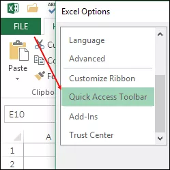
- Then, from “Choose commands from” select “Commands Not in the Ribbon”.
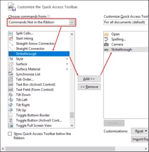
- After this, select “Strikethrough” from the list and add it to the QAT.
- At last, click OK.
Now an icon of QAT is shown and you can apply strikethrough with a single click.

Also ,this button works if you want to apply it to a particular part of a text and on multiple cells.
Apply Strikethrough from Format Option
As I said there is no direct option in Excel for strikethrough, but actually, there’s an option that you can access from format options. This is what you need to do.
- At first, select all the cells on which you want to apply it.
- After this, use shortcut key ctrl + 1 to open the format options.
- In the font tab, tick marks the strikethrough option.
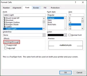
- Then , Click OK.
It works the same as other options. You can apply it on multiple cells and on the partial text. Want to know the best part? You can easily access other formatting options which are nowhere on the ribbon through the same.
Run a VBA Code to Apply Strikethrough
Macro codes work like a charm and, if you want to use a VBA for strikethrough here is the code for you.
Sub addstrikethrough()
Dim rng As Range
For Each rng In Selection
rng.Font.Strikethrough = True
Next rng
End Sub
The above code would help you to apply strikethrough on selected cells. You can also assign it into a shape to create a button.
Use Conditional Formatting to Apply Strikethrough
Conditional formatting is one of the best ways to apply formatting in a latest way. Given below is checklist where I have used a check box with conditional formatting to apply strikethrough.
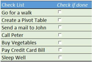
Whenever you tick a check box, the text in the corresponding cell will get a cut-through line. Here’s how you can do this.
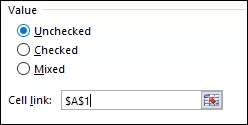
- Firstly , insert a check box in the worksheet.
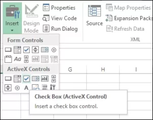
- Second, link to cell A1 and change the font color of A1 to white.
- After that select cell B1, go to Home Tab → Styles → Conditional Formatting → New Rule.
- Then Select the “Use a formula to determine which cell to format” option.
- Enter =IF(A1=TRUE,TRUE,FALSE)in the formula input bar.
- Now, click on the format option and select the strikethrough.
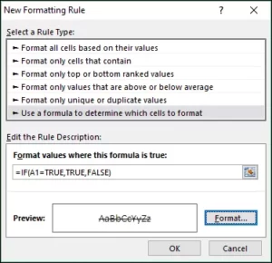
- At last ,click OK twice.
Now, whenever you tick the checkbox, the text in the cell will get automatically cut line on it.
[Bonus Tip] Apply Strikethrough in Excel Online
If you use the Excel web app then you must be happy because there is an option thereon Ribbon which you can use to apply strikethrough.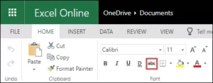
Remove Strikethrough from a Cell
It is really easy to remove strikethrough from a cell. By using the shortcut key (Control + 5) again. Important Note: If you have applied it through conditional formatting then you cannot remove it with the shortcut key unless you remove the entire formatting from the cell.
Conclusion
You can also copy-paste strikethrough from one cell to another cell using format painter. So, that’s the whole story about applying strikethrough in Excel. You have 5 + 1 different methods for this and all are easy to apply. I hope this tip will help you get better at Excel.

![Apply Strikethrough in Excel [Shortcut + Command]](https://xlsxtemplates.com/wp-content/uploads/2022/05/Apply-Strikethrough-in-Excel-Shortcut-Command-1024x576.png)
