You have dates in the column and you want to highlight all the dates which are between the range of two dates.
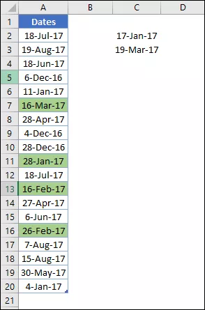
Let’s say you have a start date of 17-Jan-2017 and an end date of 19-Mar-2017, and from the dates column, you want to highlight all the cells in which date is between these two dates.
For this, the easiest way is to use conditional formatting. You can use a formula based on AND and DATE functions.
Just need to create a new rule in conditional formatting with this formula. Let’s follow these steps.
Table of Contents
Suppose, you have dates in the column and you want to highlight all the dates which falls between two date ranges.
For say you have a start date of 17-Jan-2021 and an end date of 19-Mar-2021, and from the dates column, you want to highlight all the cells between these two dates.
For this, the easiest way is to use conditional formatting. You can use a formula of AND and DATE functions.
You just need to create a new rule in conditional formatting with this formula. Let’s follow these steps.
Steps to use CF to Highlight Dates Between Two Dates
- First of all, select the range or column (A2:A20) where you have dates.
- Now, go to Home Tab ⇢ Styles ⇢ Conditional Formatting ⇢ New Rule.
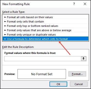
- From here, in New Rule window, select “Use a formula to determine which cell to format”.
- After that, in formula input bar, enter below formula.
- Finally, select a color from formatting option to apply to cells.
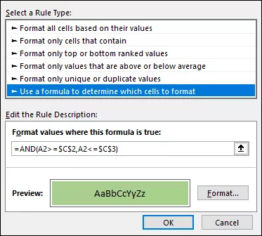
- In the end, click OK.
Once you hit OK, all the cells where dates are within the range which you mentioned will get formatted with the color you have specified.
How this CF formula works?
AND function can take more than one condition and returns TRUE if all the conditions are TRUE, else FALSE.
So when you use this formula in conditional formatting it checks the date in the cell and returns TRUE if that date is within the date range. With that TRUE, conditional formatting apply color to all the cells with dates.


