![How to CONCATENATE a RANGE of Cells [Combine] in Excel](https://xlsxtemplates.com/wp-content/uploads/2022/07/How-to-CONCATENATE-a-RANGE-of-Cells-Combine-in-Excel-1024x576.png)
The best way of combining text from different cells into one cell is using the transpose function with concatenating function.
Look at the below range of cells where you have a text but every word is in a different cell and you want to get all of them in one cell.
Below are the steps you need to follow to combine values from this range of cells into another cell.
- In B8, insert the following formula and do not press the enter key.
- =CONCATENATE(TRANSPOSE(A1:A5)&” “)
- Now, you can just select the entire inside portion of the concatenate function and press F9. It will convert it into an array.
- After that, remove the curly brackets from the starting to the end of the array.
- In the end, hit enter button.
 That’s all.
How this formula works
In this formula, you will use TRANSPOSE and space in the CONCATENATE. When you convert that reference into hard values it returns to an array.
In this array, you have the text from each cell and a space between them and when you hit enter key, it combines all of them together.
Fill justify is the most unused but most powerful in Excel. And, whenever you need to combine text from different cells you take help of it and use it.
The best thing is that you need a single click to merge the following texts. Have a look at the data provided below and follow the steps.
- at first, make sure to increase the width of the column where you have text.
- Secondly, select all the cells.
- At last, go to the Home Tab ➜ Editing ➜ Fill ➜ Justify.
This will merge the present texts from all the cells into the first cell of the selection.
If you are using Excel 2016 (Office 365), there is a function known as “TextJoin”. It will make it easy for you to combine the texts from different cells into a single cell.
Syntax:
TEXTJOIN(delimiter, ignore_empty, text1, [text2], …)
- delimiter a text string to use as a delimiter.
- ignore_empty true to ignore blank cell, false to not.
- text1 text to combine.
- [text2] text to combine optional.
how to use it
To combine the values given below, you can use the formula:
=TEXTJOIN(” “,TRUE,A1:A5)

Power Query is a fantastic tool and we all love it. Make it sure to check out this tutorial (Excel Power Query Tutorial). You can also use it for combining the text from a list in a single cell. Below are the steps.
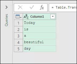
- Select the range of the cells and click on “From table” in data tab.
- It will edit your following data into Power Query editor.
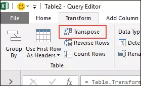
- Now from here,you have to select the column and go to “Transform Tab”.
- From the “Transform” tab, go to the Table and click on “Transpose”.
- For this, you have to select all the columns (select first column, press and hold shift key, click on the last column) and press right click on the mouse and then select “Merge”.
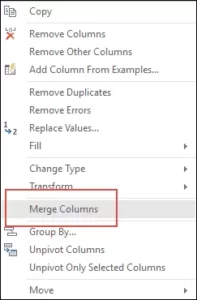
- After that, from Merge window, select space as a separator and also select the name the column.

- In the end, press OK and click on the “Close and Load”.
Now you will have a new worksheet in your workbook with all the texts present there in a single cell. The best thing about using Power Query is that you don’t need to do this setup again and again.
When you update the old list with a new value you just need to refresh your query and it will add that new value in the cell and it’s that easy.
If you want to use a macro code for combining texts from different cells then we have something for you. With this code, you can combine your texts in no time. All you need to do is, select the range of cells where you have to text and run this code.
 Sub combineText()
 Dim rng As Range
 Dim i As String
 For Each rng In Selection
 i = i & rng & " "
 Next rng
 Range("B1").Value = Trim(i)
 End Sub
Make sure of specifying your desired location in the code where you want to combine your text.